Eli can retire Part XIII - Tom Segalstad is an old buddy

In which the EPA explains to Judith Curry why Tom Segalstad is wrong, wrong, wrong.

Comment (2-3):
Several commenters state that CO2 has a short lifetime in the atmosphere (0711.1, 0714.1): for example, a commenter (1616) claims that the lifetime of CO2 can be at most 20 years based on the 12% annual exchange of CO2 with the surface ocean and 10% exchange between the surface and deep ocean as shown in the National Aeronautics and Space Administration (NASA) carbon cycle diagram, and two commenters (3440.1, 3722) state that the overwhelming majority of scientific papers support a residence time of seven years in contrast to the TSD and IPCC. Several commenters (e.g. 3722) cite Professor Segalstad who has stated, based on his work on CO2 residence times (Segalstad 1997), that the assumption of a 50- to 200-year lifetime by IPCC results in a “missing sink” of 3 Gt of carbon a year, which is evidence that IPCC is mistaken.

Another commenter submitted Essenhigh (2009), which developed a box model and also found that the lifetime of CO2 was on the order of a few years.

Response (2-3):
EPA reviewed the information presented, as well as the work by Segalstad, and finds that it does not address the lifetime of a change in atmospheric concentration of CO2, but rather the lifetime in the atmosphere of an individual molecule of CO2. These are two different concepts. As stated in the First IPCC Scientific Assessment, “The turnover time of CO2 in the atmosphere, measured as the ratio of the content to the fluxes through it, is about 4 years. This means that on average it takes only a few years before a CO2 molecule in the atmosphere is taken up by plants or dissolved in the ocean. This short time scale must not be confused with the time it takes for the atmospheric CO2 level to adjust to a new equilibrium if sources or sinks change.

This adjustment time ... is of the order of 50–200 years, determined mainly by the slow exchange of carbon between surface waters and the deep ocean” (Watson et al., 1990). The magnitudes of these large balanced sources and sinks are addressed in response 2-2, and are similar to those represented in the NASA carbon cycle diagram. Newer research has only extended and confirmed this statement from the first IPCC assessment report (Denman et al., 2007). A recent approximation for this perturbation lifetime is sometimes represented as the sum of decay functions with timescales of 1.9 years for a quarter of the CO2 emissions, 18.5 years for a third of the CO2, 173 years for a fifth of the CO2, and a constant term representing a nearly permanent increase for the remaining fifth (Forster et al., 2007).

The “missing sink” that was referred to by a commenter is also addressed in response 2-2, and is now called the “residual land sink.” The magnitude of this sink is about 2.6 Gt of carbon per year, with significant uncertainty. Denman et al. (2007) included a hypothesis that a portion of this sink is due to the increased growth of undisturbed tropical forest due to CO2 fertilization, but the carbon accumulation of natural systems is hard to quantify directly. The uncertainty in determining the size and nature of this residual sink does not contradict the assessment literature conclusions about the perturbation lifetime of CO2 concentration changes in the atmosphere, but is reflected in the carbon cycle uncertainty for future projections of CO2 (see responses regarding carbon cycle uncertainty in Volume 4 on future projections).

The box model in Essenhigh (2009) is clearly flawed: the results from this model as reported in the paper include a lifetime for CO2 containing the 14C isotope that is a factor of 3 different from the lifetime of CO2 containing the 12C isotope. This difference in lifetimes is not scientifically compatible with the immense difficulty involved in isotope separation. The model assumes that each “control volume” (each volume represents either the ecosystem, the surface ocean, or the deep ocean) is perfectly mixed, which is contrary to the observations of oceanic CO2 which show that storage of carbon in the ocean is only at 15% of the equilibrium value, and that the mixing time between the surface ocean and intermediate and deep oceans is on the order of years to centuries (Field and Raupach, 2004). Additionally, the paper uses only historical fossil fuel emissions of CO2, without including land use change CO2, and contains the same confusion about “residence lifetime” and “adjustment lifetime” that has been addressed above.

A common analogy used for CO2 concentrations is water in a bathtub. If the drain and the spigot are both large and perfectly balanced, then the time than any individual water molecule spends in the bathtub is short. But if a cup of water is added to the bathtub, the change in volume in the bathtub will persist even when all the water molecules originally from that cup have flowed out the drain. This is not a perfect analogy: in the case of CO2, there are several linked bathtubs, and the increased pressure of water in one bathtub from an extra cup will actually lead to a small increase in flow through the drain, so eventually the cup of water will be spread throughout the bathtubs leading to a small increase in each, but the point remains that the "residence time" of a molecule of water will be very different from the "adjustment time" of the bathtub as a whole.

This analogy does not hold for other GHGs: methane, HFCs, and N2O are actually destroyed chemically in the atmosphere, unlike CO2 where the carbon is not destroyed but merely shifted from one reservoir to another, and therefore the residence lifetime of these gases is fairly close to the adjustment lifetime of their concentrations in the atmosphere.

Similarly, any given molecule of CO2 is only expected to stay in the atmosphere for a few years before it moves into the oceans or ecosystem, but the change in atmospheric concentration due to combustion of fossil fuels can persist for much longer. Indeed, because the oceans and ecosystems are finite, some small fraction of CO2 emissions will have a perturbation lifetime in the atmosphere of thousands of years (Karl et al., 2009).

Next

The Judith Curry Debunking Room is open

The bunnies have been looking for a new project and Judith Curry has been looking for answers. She pawed her way through the Heartland International Climate Change presentations

Interpreting the surface historical temperature record.

Pat Michaels: slides 30-32, changes in the CRUT temp anomalies with time, these are unexplained

Your name here

Craig Loehle: historical surface temperature records. Makes the same point as Pat Michaels about strange changes in subsequent versions of CRUT temperature analysis. Makes PDO type arguments.

Nebuchadnezzar: It looks as if Craig Loehle has inadvertantly switched in global land surface air temperature (i.e land only) for global surface temperature (land and sea combined) in slides 7 thru 9 and into the conclusion of 10.

The red line (2010) is land only (aka crutem3). The black line (2008) is land and sea (aka hadcrut3).

That would explain - very simply - the 'unexplained' change between 2008 and 2010. Easy mistake to make.

global land surface air temperatures are here:
http://hadobs.metoffice.com/crutem3/diagnostics/global/nh+sh/

global surface temperatures (land and sea) are here:
http://hadobs.metoffice.com/hadcrut3/diagnostics/global/nh+sh/

Nick Stokes provides a nice graph of of hadcrut3gl (land/ocean) vs crutem3 (land only)

Roy Spencer: inadequacy in urban heat island analysis.

Your name here

Joseph D’Aleo: describes a number of global data base issues. The impact of these issues (individually and collectively) on the global temperature data record is unknown.

Ron Broberg has a long post on this shooting down the many claims.
http://rhinohide.wordpress.com/2010/05/24/daleo-at-heartland-an-apple-a-day/

Christopher Monckton: see slides 12-14 re trends in the historical temperature record. Hard to disagree with his analysis that the “accelerating trend of global temperature increase” in IPCC (2007) is based upon faulty statistical analysis.

By way of Joe Romm, a loooong presentation by John Abraham, tearing Chris a new one. This link will, without a doubt cause Kloor to sputter, but Judith Curry might benefit by viewing it.

Chip Knappenberger: Modeled vs observed temperature trends over the last decade. Good study with appropriate analysis methods as far as I can tell.

Nick Stokes comments on this at moyhu. Chip and James should have waited a few months. James say a few things

Ross McKittrick: tropospheric temperature trends. Discrepancies between models and observations. This issue is not going away, it is gaining more traction. Santer (2008) statistical methods are criticized.

Your name here

McIntyre:(video) the “decline”. Yes I’ve read DeepClimate’s analysis, but it does not detract from McIntyre’s analysis that this is not good scientific practice.

This is almost silly. How many reports are needed to point out that a) the trick was described in the literature along with the reasons for it. b) there was no dishonesty.

Note: David Douglass made a presentation, but it is not available

On occasion one is lucky

Feedback issues:

Lindzen: usual stuff, but he takes on a new issue, Arctic sea ice. He commits a howler by claiming that summertime loss of arctic sea ice cannot be related to warming since the summertime ice surface temperature has remained constant for decades (he forgot about the latent heat of melting).

Shall someone pile on

Roy Spencer: cloud feedback issues, mentions a new paper coming out in JGR.

Any takers

George Kukla: some issues related to long time scale feedback processes. global cooling in early interglacials, and global warming in early glacials.

Your name here

Bill Kinimonth: coupling of water vapor and ocean surface latent heat feedbacks. Aspects of his actual analysis are not correct, but he raises an important issue in terms of likely climate model deficiency in this regard.

Your name here

Arctic sea ice:

Fred Goldberg: historical ice observations in the Arctic. Describes low amount of arctic sea ice in the 1920’s. Projects future arctic sea ice based on natural variability.

Your name here.

——-beyond this point I have no particular expertise, but think these presentations may be of interest, and I personally would be interested in blogospheric discussions on these papers.

Other contributions welcome

Solar variability:

Abdussamatov: An interesting new twist, associated with cyclical variations in the radius of the sun. Predicts beginning of a new little ice age in 2014, with temperatures in 2100 about 1.2 degrees cooler than current owing to solar forcing. His theories are linked to recent changes observed other planets. The only debunk I’ve seen was unconvincing (by chuck long) about observations of global dimming/brightening.

Your name here, but the finding of new "cycles" is a perennial, esp with Solar Cycle 24 starting to cook.

Victor Herrara: solar cycles. Seems to be onto the same thing as Abussamatov, 120/240 year cycles.

Your name here

Carbon issues:

Craig Idso: ocean acidification. I’m not an expert in this area, but these arguments should be examined, particularly the Tans (2009) paper. A quick google blogs search did not identify a debunk of this paper.

A good example about why to count your fingers after you deal with these folks. As Steve Bloom points out Idso used only one of the two scenarios that Tans set forth, the low total emissions one where emissions peak in 2029 and CO2 peaks at 500 ppm in 2069. The second one, Scenario B as it were, had emissions peaking in 2044 and peak CO2 mixing ratios of 600 ppm in ~2075. In both cases the mixing ratios decay slowly over the next four hundred years to about 2/3 their peak value.

Futher, when Idso compares Tans' estimates of changes in ocean pH, he somehow neglects to point out that the IPCC considered scenarios where the mixing ratio was much higher than 600 ppm peak, which, of course, meant that the pH change would be much more, but Idso does use the difference to imply that the IPCC is wildly off. Count your fingers folk.

Idso then looks at the results of experiments that studied the effect of pH change on various parameters. While Eli is no expert here, it is clear that the effect will vary strongly with species, for example, most species that build shells (calcification) will be strongly affected in a negative way, although there are a few which will be able to handle pH changes in the range predicted by Tans for 500 or 600 [CO2] peaks. The effect of lumping everything together is to miss the enormous challenges for individual species, some of which we depend on.

Tom Segalstad: CO2, challenges measurements and attribution to fossil fuels. Addresses the “mysterious missing carbon sink.” Haven’t been able to find an online debunk.

M- O'Neill, B.C., Oppenheimer, M. and S.R. Gaffin (1997) Measuring time in the greenhouse, Climatic Change 37, 491-503.

Also, the EPA TSD (see post above this one)

Sea level rise:

Nils Axel Morner: local sea level rise. Discusses the complexity of issues that go into determining local sea level rise. Claims no sea level rise in the Maldives, Tuvalu, Vanuatu, Bangladesh, Qatar, Venice, NW Europe. Questions calibration of satellite altimeters. I don’t know much about this topic, would be interested in further discussions of this.

Do some of the Nordic Bunnies want a whack at Uncle Nils?

M contributes

Ah, Morner who labels observations by other people "model results" and "personal calibrations" but his own cherry picked selection of tide gauges and made-up numbers are the only real "observations".

Sources counter to Morner: From Skeptical Science on sea level rise and
Woodworth, "Have there been large recent sea level changes in the Maldive Islands" (Global and Planetary Change 2005)
Church

Also, Morner's supposed "10 mm/century upper limit" is contrary to the estimates for SLR during meltwater pulse 1a:

Bob Carter: another paper stressing the importance of focusing on local sea level rise at coasts rather than global average values

When you got nothing, move on.

Contributions?

Slippery slopes

Sometimes the title is the reason for posting. This is one such case.

The Heartland Conference on Climate Misleading has given us two contenders: Don Easterbrook, who picks the beginning of the temperature anomaly curve as 2000 and the end as 2009 to fake the decline, as Tim Lambert points out, or is it hide the incline, and then James Taylor who does the same for snow cover. Friend Taylor shows up at MT's place to defend his honor, decides, it's not worth the effort, picks up his few marbles remaining and goes home. MT plays a round of nyah nyah.

Offend everyone day

Stoat has declared offend everyone day. Who is Eli not to take part?

Whan that Aprill with its cold snap sorta

The colde of Marche hath perced to the rote,
And bathed Arctic veynes is swich new ice,
Of which denial engendred is the flour;

Comes monthe May with its swete breeth
Inspired hath in every holt and heeth
The tendre currents, and the yonge sonne
Melts the ice and floats the boatas

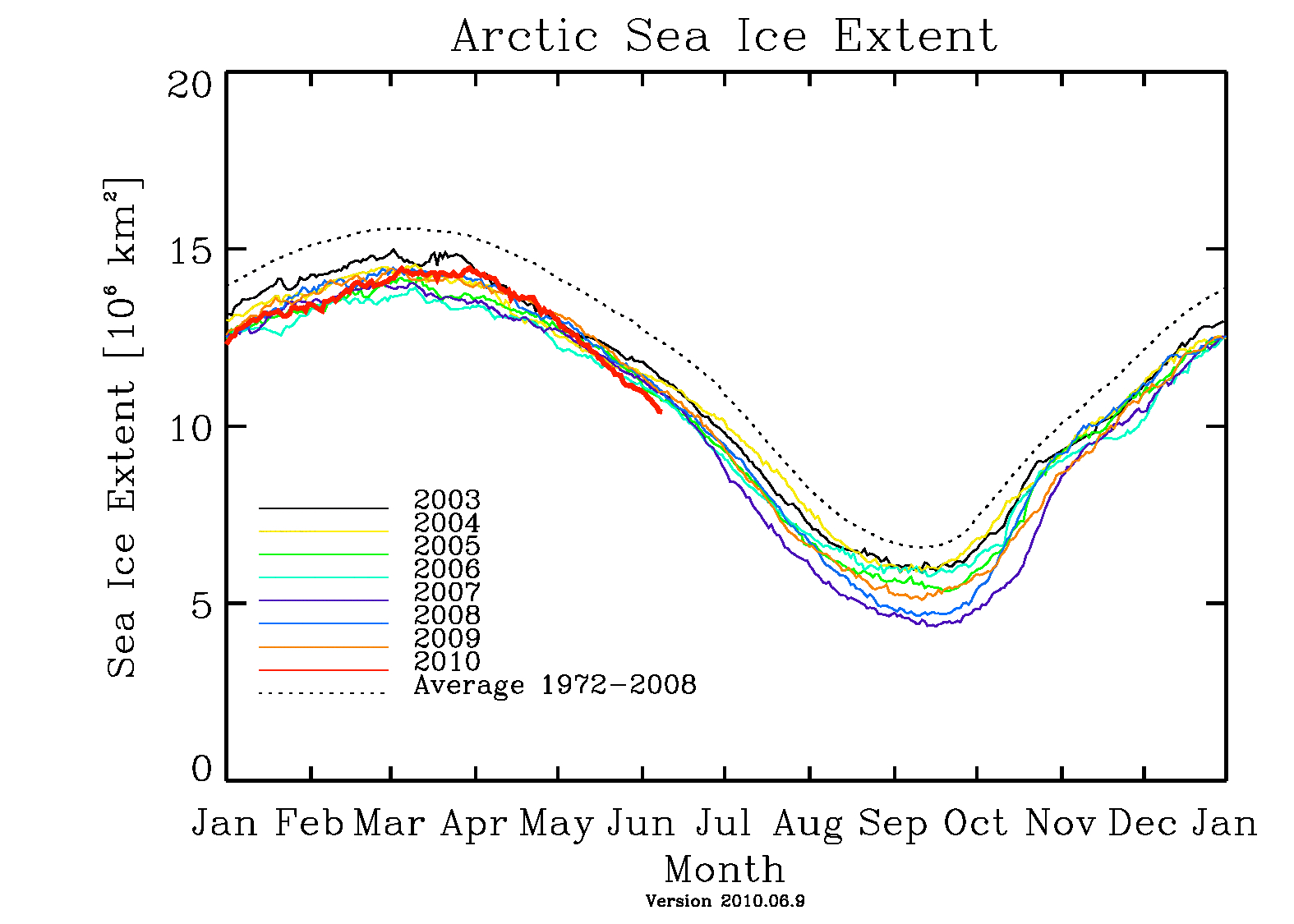
Its Arctic Ice Blogging time folks, with a vengence. There is a rapid breakup, the somewhat misleading ice buildup in the sub-Arctic Sea of Okhotsk and the Baltic is going, Hudson's bay is clearing and it looks like another banner year for shipping in the Northern Passage. The Chinese fleets are setting sail as we wait. (The IUP site goes to sleep at night be back tomorrow)

UPDATE: The images now are for 6/10/2010



Eli is trying to figure out what all the little flecks in the map are when you blow it up, but still the ice is thinning rapidly, and if we go to the tape. . .



the ice extent is now under 2007 and approaching the all time low for May.

Oh yeah, as Stoat points out there is

a) either something rotten in Alabama or
b) the upper atmospheric hotspot is taking a bow

and it is the hottest April ever, or at least since we got thermometers.

More arrogant physicists

(Notice to the uninterested, the lede is significantly buried here, but this is a blog, not a newspaper)

Eli and the seven bunnies are quite into arrogant physicists, one of them, Arthur Smith, even spent some time laying the species out.

In general though, physicists have good reason to be arrogant. Each of us in the intellectual world is like an armed policeman. A certain swagger is justified, we feel confident we have the tools to handle any situation. A problem asserts itself, and we walk in with the self-assurance of those who have tackled thousands of similar cases in the past. For a really challenging problem we know how to put out a call for reinforcements. One all-purpose tool is reductionism - breaking a problem into smaller more comprehensible pieces, and then tackling those one by one. . . .

But sometimes that arrogance and self-assurance and collection of intuitions lead us, or at least a few of us, astray. We forget that there are other smart people in the world, who have been thinking about their limited problem for a lot longer and perhaps have a deeper understanding than we give them credit for. We jump in with our simplified models and ideas and then wonder why they don't find them helpful. Or we too deeply trust the intuition of a colleague who has been often right before or who we trust for other reasons, but in a particular instance has not put in the effort to properly understand the problem, and ends up only embarrassing themselves, and us by association.

Eli, of course, having been demoted to mere chemist by the real physicists Gerhard Gerlich, Ralf D. Tscheuschner is not qualified to comment on these matters, other than to note that their recent diatribe in IJMPB

One should keep in mind that we are theoretical physicists with experimental experience and, additionally, a lot of experience in numerical computing. Eli Rabett and Joerg Zimmermann, for example, are chemists. We are not willing to discuss whether they can be considered as laymen in physics, in particular laymen in thermodynamics.

Is a strong contender for the Boojum's Golden Horseshoe Award

In Dashiell Hammett’s story The Golden Horseshoe, much of the action takes place in a bar of that name in Tijuana. At one point the narrator, an operative for the Continental Detective Agency, kills a few strategic seconds by studying the decorations:

I was reading a sign high on the wall behind the bar:

ONLY GENUINE PRE-WAR AMERICAN AND BRITISH WHISKEYS SERVED HERE

I was trying to count how many lies could be found in those nine words, and had reached four, with promise of more …

Sometimes I come across an article, web posting, advertisement or other statement that makes me feel when I read it just as I imagine the Continental Op did in that Tijuana bar.

How can they possibly pack so much misinformation into such a small space?

Which kind of brings us to the almost end, with the appearance of the obfustication aka the commentary appended now to the American Physical Society's Statement on Climate Change. John Mashey spent a great deal of time tracing the attack on the the APS Climate Change Statement back to a few nests of "motivated" (Judith Curry instructs Eli not to use the words denialist, or reactionary) physicists at a few places including Princeton. Which, finally, brings Eli to the point. Jonathan Katz, Professor of Physics at Washington University, was one of those who petitioned to change the APS policy statement. Katz had previously been a member of the Institute for Advanced Studies at Princeton, and was evidently recruited for JASON at that point, something he shared with other petitioners.

JASON is a small advisory group of arrogant scientists which grew out of the Manhattan project to advise the Departments of Defense, Energy and Spooks about scientific matters. To cut to the chase, Steve Chu turned to JASON in order to get an evaluation of how to deal with the oil well blowout in the Gulf and the impending disaster. They sent a few members, including the aforementioned Dr. Katz, and as it happens, people started looking at the members' web sites.

Dr. Katz has the habit of posting essays (sub - blogging as it were) on his web site, and one of them turned out to be, well, homophobic. Dr. Katz was landed upon, and disinvited

Jonathan I. Katz, a professor of astrophysics at Washington University in St. Louis, ''will no longer be involved in the [Energy] Department's efforts'' at addressing the oil spill continuing to spread in the Gulf of Mexico, a Department spokeswoman relayed on Monday night, May 17.

The news came after what the spokesperson, Stephanie Mueller, termed ''controversial writings'' – which included a ''defense of homophobia'' – spread out over the web on Monday, writings of which she said the Department was unaware when it sought his assistance.

On May 12, Energy Secretary Steven Chu ''assembled a group of top scientific experts from inside and outside of government to join in today's discussions in Houston about possible solutions,'' according to a Department news release. Katz was one of five outside scientists noted in the release. Bloomberg News reported about the group of scientists on May 14, reporting Chu ''signaled his lack of confidence in the industry experts trying to control BP Plc's leaking oil well by hand-picking a team of scientists with reputations for creative problem solving.''

His comments about climate change incorporate the equally charming mixture of naivety, agression and arrogance that characterize physicists of a certain training, and the dénouement was about as predictable.

Perhaps we might now start a discussion of Prof. Katz's take on climate change? Eli's take on that is that the cheerful assumption that no one else was paying attention to the various ups and downs in radiative forcing over the last 150 years, is, as usual with such characters, charming.

Stumbling across campus to talk to people with a clue might have helped. Pierrehumber's Law.

Eli can retire Part XII - The commenters get something right

Another in our series, but this time the EPA and the commenters get it right

Comment (6-44):
Commenters (e.g., 2791, 10298) state their support for the Findings, noting the potential for increased stress from heat, drought, insects, and disease on plant and tree populations. Others (2599, 10081) from the western United States voice their support for the Findings and describe their experiences with hot summers and serious wildfires. Other commenters (e.g., 3421, 4748, 6894) state their support for the Findings and express concern about the effects of current and future extreme weather events on the forestry industry, including heat waves, droughts, floods, wildfires, and hurricanes. One commenter (5844) describes how projected climate impacts, particularly the increased risk of wildfire on forestry and forest biodiversity will affect him personally given his enjoyment of hiking, camping, and communing with nature in the forests of the Pacific Northwest.

A commenter (3501) states his support for the Findings, indicating that the western United States and Canada are already seeing widespread changes in the natural landscape due to climate change. Hotter temperatures are causing more frequent and persistent drought in the West, which contribute to forest fires and pine beetle infestations. A weather-related pine beetle infestation has decimated millions of acres of forest in the western United States Western US and Canada. At the current rate of destruction, 80% of the forests of British Columbia will have been destroyed within five years and the rest of the West will lose 50% of its forests by mid-century. The forest fire season in the West is now 78 days longer than 25 years ago and it is well recognized that our forest fires have become more frequent, more intense and more destructive.

Response (6-44):
We reviewed the comments provided and note they are generally consistent with the discussion of climate impacts on forestry in the TSD, although commenters do not provide specific references to support their claims. As summarized in the TSD and in our responses to previous comments in this volume, disturbances like wildfire and insect outbreaks are increasing and are likely to intensify in a warmer future with drier soils and longer growing seasons.

The Technical Support Document provides the background for this, of which Eli will quote a bit

10(d) Insects and Diseases
Insects and diseases are a natural part of forested ecosystems and outbreaks often have complex causes. The effects of insects and diseases can vary from defoliation and retarded growth, to timber damage, to massive forest diebacks. Insect life cycles can be a factor in pest outbreaks; and insect life cycles are sensitive to climate change. Many northern insects have a two-year life cycle, and warmer winter temperatures allow a larger fraction of overwintering larvae to survive. Recently, spruce budworm in Alaska has completed its life cycle in one year, rather than the previously observed duration of two years (Field et al., 2007). Recent warming trends in the United States have led to earlier spring activity of insects and proliferation of some species, such as the mountain pine beetle (Easterling et al., 2007).

During the 1990s, Alaska’s Kenai Peninsula experienced an outbreak of spruce bark beetle over 6,200 square miles (16,000 km2) with 10 to 20% tree mortality (Anisimov et al., 2007). Also following recent warming in Alaska, spruce budworm has reproduced farther north reaching problematic numbers (Anisimov et al., 2007). Climate change may indirectly affect insect outbreaks by affecting the overall health and productivity of trees. For example, susceptibility of trees to insects is increased when multi-year droughts degrade the trees’ ability to generate defensive chemicals (Field, et al., 2007). Warmer temperatures have already enhanced the opportunities for insect spread across the landscape in the United States and other world regions (Easterling et al., 2007).

The IPCC (Easterling et al., 2007) stated that modeling of future climate change impacts on insect and pathogen outbreaks remains limited. Nevertheless, the IPCC (Field et al., 2007) states with high confidence that, across North America, impacts of climate change on commercial forestry potential are likely to be sensitive to changes in disturbances from insects and diseases, as well as wildfires.

The CCSP report (Ryan et al., 2008) states that the ranges of the mountain pine beetle and southern pine beetle are projected to expand northward as a result of average temperature increases. Increased probability of spruce beetle outbreak as well as increase in climate suitability for mountain pine beetle attack in high-elevation ecosystems has also been projected in response to warming (Ryan et al., 2008).

Climate change can shift the current boundaries of insects and pathogens and modify tree physiology and tree defense. An increase in climate extremes may also promote plant disease and pest outbreaks (Easterling et al., 2007).

And so, we get to the scary bits To be continued. . .

The very dry, very adiabatic lapse rate

Over at the real Pielke Sr. web site aka Tony Watts plays scientist, Steven R Goddard misunderstands what the dry adiabatic lapse rate is and tries to claim that the hothouse Venus is strictly a gravitational effect. Nick Stokes and Leonard Weinstein try and set him right. The Bunny got a comment through (after a considerable delay) but Watts is blocking Eli's further words of wisdom over there, and besides the same thing has broken out on moyhu and Real Climate, where Richard Steckis touched it off

The essential argument is that the heating of the Venusian atmosphere occurs through adiabatic processes and not through absorbance of IR by GHGs.

[Response: Since 'adiabatic' means without input of energy it seems a little unlikely that it is a source of Venusian heating. - gavin
Comment by Richard Steckis — 7 May 2010 @ 12:19 PM

and

Stephen Baines says:
7 May 2010 at 10:44 PM
“@ RS “As for Gavin’s comment re: pseudo-science, I guess it is only pseudo-science when it disagrees with your pre-conceived ideas about Venusian climate.” 

If by preconceived ideas, you mean ideas conceived and tested by scientists over more than a century of prior research, I think he would agree.” 

A century of research can be toppled by one experiment. So do no hang your petard on the fallacy that a century of research is an unbreakable bulwark of truth. 

[Response: If you think a century of science is going to be toppled by obviously ignorant blog posts on WUWT, you are very mistaken. There is a big difference between coming up with new insights that cause a reevaluation of current paradigms and just getting very basic physics wrong and misapplying completely other bits of physics. Goddard and Motl are engaged in the latter, not the former. - gavin]

Comment by Richard Steckis — 8 May 2010 @ 9:22 PM

There is more but you get the feeling, so let Eli have his say.

It's called the dry adiabatic lapse rate, which means that it is an idealization where the energy flow into and out of any packet of air is balanced. That is what Gavin was getting at.

The surface temperature is fixed by a radiation balance between incoming solar and out and incoming IR. The second, colder endpoint is some place up there where something else happens to break the adiabatic condition, for example ozone absorption starting to kick in at the top of the Earth's troposphere. For a planet with an atmosphere and no greenhouse gases, pretty much the temperature of space.

That leaves gas rarification/compression driven by gravitation as the mechanism for setting the atmospheric temperature profile. It is not saying that radiative energy flow is negligible, just that it is balanced.

What does the lapse rate determine? Looking at extremes is useful. If the surface is at absolute zero the thickness of the atmosphere (at least for an ideal gas) would be zero. What if the surface were at infinite temperature. Then the height of the atmosphere would be infinite also. From this, we conclude that the height of the atmosphere is determined by the lapse rate and the surface temperature
There are, of course, a few other things to consider. First, the dry adiabatic lapse rate is not 10 K/km for every atmosphere. For example it is 4.5 K/km on Mars and 2.0 K/km on Jupiter. Better put it is the ratio of the local gravitational constant divided by the specific heat (in J/(kg-K) or g/Cp. For the case of Venus, where the surface and the atmosphere are very hot, we have to account for the contribution of molecular vibrations to the specific heat, which will change with temperature and thus with altitude.

The lapse rate does not set the surface temperature, which is determined by the solar radiation absorbed at the surface and the IR re-emitted by greenhouse gases in the atmosphere.

End

Gavin Schmidt can retire Part I - The EPA sticks it to Steckis

Caerbanog brings word that Richard Steckis has been channeling Steve Goddard at the Sr. Pielke's vanity site WUWT, about Venus at Real Climate and Gavin is NOT amused. However, as Cthulhu has pointed out, the EPA has already answered the off earth questions. Sometimes, you just have to look it up

Comment (3-49):
A commenter (2210.1) states that Venus is not an example of the greenhouse effect but is merely warmer because it is closer to the sun. Another commenter (2210.5) attributes Venus' warmth to higher atmospheric pressure because compression causes temperature increases (for example, this occurs when inflating a bicycle tire, due to the proportional relationship between pressure and temperature represented in the ideal gas law, pV=nRT, i.e., pressure times volume equals amount of gas times temperature times a constant), and that a 95% CO2 atmosphere is actually cooler than a 100% biatomic atmosphere would be.

Response (3-49):
Venus is warmer than the Earth both because of the greenhouse effect and because of its distance to the sun; in contrast, Mercury is cooler than Venus despite being even closer to the sun. Were Venus’ atmosphere to be transparent to radiation, then the surface temperature of Venus would be determined only by the blackbody radiation of the surface, and the pressure of the atmosphere would not change this equilibrium temperature. There is a large body of literature on Venus’ climate; one example is Bullock and Grinspoon (2001)—all of which show that CO2 is a significant contributor to the planet’s warmth.

Because volume is not held constant, it is not appropriate to use the ideal gas law to determine the temperature on the surface of Venus based only on knowledge about its pressure. Therefore, the scientific literature shows clearly that the temperature of Venus is an example of a greenhouse effect, in contrast to the assertion by the commenters.

Comment (3-51):
One commenter (3013) mentions Mars and states that even given the lower atmospheric pressure, his calculation shows that it has twice as much CO2 as Earth, and further claims that the National Aeronautics and Space Administration (NASA) found that the even with this high CO2 concentration, the atmosphere of Mars does not retain heat.

Response (3-51):
The commenter did not provide any evidence for his claim that NASA has found that the atmosphere of Mars does not retain heat. Mars does have an atmosphere that is mainly carbon dioxide, but because of the low atmospheric pressure, it is only 16 times the quantity of carbon dioxide on Earth. At the same time, it receives less than 45% as much sunlight, so the increased radiative forcing from the CO2 is not sufficient to make up for the decrease in solar insolation. Thus, the commenter’s claim that the atmosphere of Mars does not retain heat is not consistent with the scientific literature.

Comment (3-39):
A few commenters (0717, 4003) noted that there is warming on other planets, mentioning Mars, Jupiter, and Pluto, and stated that this was evidence for the solar cause of global warming.

Response (3-39):
The commenters did not provide any peer-reviewed literature to support their argument. One indication that Mars is warming was a retreat of the South Polar Cap, but Colaprete et al. (2005) discuss the fact that the South Polar Cap is unstable, and that it is therefore difficult to extrapolate short-term changes in the cap to a long-term global trend. Martian climate is also influenced by non-solar mechanisms such as positive feedbacks between albedo changes and changes in dust storms (Fenton et al., 2007).

Therefore, it is neither clear that Mars is warming nor that the warming is solar induced. The climate on Jupiter is dominated by the dynamics of the massive standing vortices on the planet (Marcus, 2004), and solar energy is a less significant contribution to the temperature of Jupiter than it is for Earth. It is also unclear whether the warming of Jupiter is global or regional.

The changes in Pluto’s atmosphere have been detailed in Elliot et al. (2007). The basic atmospheric expansion is well modeled by the frost migrations models of Hansen and Paige (1996), without requiring any solar effects beyond Pluto's seasonally changing sub-solar latitude. Because Pluto takes about 248 years to orbit the sun, Pluto’s seasons can be measured in decades. Finally, Triton is the last commonly referenced “warming” planet. The last good measurements of Triton were in 1998 (Elliot et al., 1998), and the changes in Triton's pressure have been explained by the change in Triton's subsolar latitude uncovering polar icecaps to the sun as a result of Triton's obliquity.

Therefore, there is no indication that solar variability is the cause of recent warming on any solar system body. Additionally, the lack of recent observed trends in solar insolation (discussed in responses in this section of the Response to Comments document) makes it implausible that there would be such solar induced warming trends on solar system bodies.

Δεν υπάρχει πιο

Unto us a paper is given, unto us a refutation is born

Eli has often talked about how a major strength of astronomy, ornithology and just plain botanizing as a friend puts it (didn't know lagomorphs had friends, did you), is their amateur communities. While there have always been those obsessed with the weather who operated weather stations, the emergence of digital communications and the web has integrated large numbers of stations into at least the networks of TV weathercasters, if only because the later saw it as a low cost opportunity to broaden their appeal to the local community. With significant computing power and expertise available ground truth is moving away from the professionals and toward amateurs, and even some computational work is moving in that direction.

Climate science today is showing stress from this effort. Because of politicization it will not be a smooth road. In the discussion about weather station records needing to be reduced to bits, it is obvious that there is a large crowd of folks who would take pleasure in doing this, but it is also obvious that quality control would be a horror, as some, far be it from Eli to say whom, would also like to shift the numbers up and down a bit.

The two best examples to date of participatory climate science are the Clear Climate Code Project which is attacking the cost and time issues associated with heritage code (grandfather wrote it back in the days of streaming tape and core memory) by involving volunteers (nice powerpoint presentation at the link for bunnies who would learn more), and the Oxford Climate Prediction.net, offering folk the opportunity to participate in using a simple GPS (e.g. today something that was state of the art maybe 15 years ago) to build a large ensemble of global simulations.

About a year ago, Eli gathered some readers up to produce a publishable refutation to a rather amateurish and ill tempered effort by Gehard Gerlich and Ralf Tscheuschner. The RR paper was finally accepted about three months ago, and has now appeared,

Comment on Falsification of the Atmospheric CO2 Greenhouse Effects Within the Frame of Physics, JB Halpern, CM Colose, C Ho-Stuart, JD Shore, AP Smith and J Zimmermann,, International Journal of Modern Physics B, 24 (2010) 1309-1332 doi 10.1142/S021797921005555X

and damn it, Stoat saw it first although all the parents were waiting for it. As far as Eli knows, this is the first time a scientific paper was written out in the open on a blog, with multiple participants who volunteered their time. You can follow the saga by searching Rabett Run using the keyword "Gerlich" although you will also have the pleasure of reading comments upon the original comments, including a comment by the EPA. While our comment is behind a paywall, feel free to look at an earlier version (it went through 15 drafts) and two rounds of reviews (Hi Gerhard) at Rabett Run Labs.

Of course, there is a reply by Ralf Tscheuschner and perhaps Eli will get to that. He anticipates a visit from the good Dr. Kramm trying to break his lance on the bunny, etc.

Finally, a good word for a new effort by one of the authors, Chris Ho-Stuart to establish a discussion form on the physics of climate,

Our aim is to support substantive discussion of the science of climate, especially the underlying physics. We focus on ideas that have been published in the mainstream scientific literature. This still allows for all kinds of competing ideas to be considered, while hopefully avoiding distraction from ideas that have no credible basis.

which starts with a discussion, of what else, our discussion of the Gerlich and Tscheusner paper. Chris' ambition is to replace the late (it became too controversial for them) physicsforum climate discussions. Eli has added a link on the blogroll.

This is the Environmental Protection Agency, Division of Answering Ignorant Questions from Belligerent Know-it-alls, Climate Sector. Can I help you?

Thanks to MT, for an even better way of labeling the on-going Eli used to be able to retire threads. Today we start the EPA blonks Plimer series

Comment (2-17):
A commenter (11454.1) provided quotes from Heaven and Earth (Plimer, 2009) claiming that CO2 was higher in 1942 than today based on the “Pettenkofer” method, and denigrating the use of infrared spectroscopy in modern CO2 analysis due to a lack of validation against the Pettenkofer method. Another quote provided from the same source disparaged the Mauna Loa data because only 18% of the raw data is used in statistical analyses.

Response (2-17):
We have reviewed Plimer’s book, and find that it has not been peer-reviewed or undergone any objective and thorough evaluation of its claims. The Pettenkofer method is a chemical method for determining CO2 concentrations in the atmosphere. Regardless of its accuracy, if used in inappropriate locations such as in or near towns or other areas that have high local CO2 concentrations, the Pettenkofer method will not result in a measurement of the global background concentrations (in contrast to the current measurement stations such as the Mauna Loa station, which are carefully placed in remote locations). See response 2-4 regarding CO2 concentrations reported by Beck (2007).

We find that the use of infrared spectroscopy for CO2 measurements has been validated extensively. Not only are infrared spectrometers used in scientific laboratories around the world, but the instruments used for measuring global background CO2 concentrations are regularly calibrated against CO2 samples that have been assessed by manometric measurements, involving condensing and separating CO2 and N2O from the remainder of the air and using a gas chromatograph to determine the CO2 to N2O ratio in the liquefied sample. This manometric procedure is estimated to have an accuracy of 0.07 ppm. Therefore, we find no support for the commenter’s objections to the use of infrared spectrometers.

With respect to Plimer’s claim that the Mauna Loa dataset was selectively edited in order to make an upward-trending CO2 curve, NOAA provides a rigorous description of the process used to measure, calibrate, and report the data from Mauna Loa at http://www.esrl.noaa.gov/gmd/ccgg/about/co2_measurements.html (Tans and Thining, 2008). The data are all archived, including any raw data that are not included in the final reporting. In contrast to Plimer, we find that 52% of the hourly data from 2008 were retained, consistent with the statement from NOAA that there is an average of 13.6 retained hours per day (57%) over the entire record. We also find that, with the exception of the 15% of the data that were recorded as “instrument malfunction,” the average of the included data in 2008 was within 0.2 ppm of the excluded data, contrary to the assertion by Plimer that selective editing was used in order to change the trend. These data have been extensively reviewed, published in the peer-reviewed literature, and ultimately also used by the broad climate change assessment community. In addition, the data from Mauna Loa are consistent with data collected at remote sites around the world, as well as with samples collected in air flasks and measured at a central site rather than on location (these flask data are on average within 0.11 ppm of the infrared analyzer data).

The confidence that the modern CO2 record gathered around the world represents accurate measurements of the global background CO2 concentration is therefore extremely high, in contrast to the northern European data collected by the Pettenkofer method in 1942. Therefore, we determined that the assertions of the commenter and the underlying source are not consistent with the current scientific literature.

Gibts nicht mehr

Rabett Reader

Stephen Lewandowsky and John Quiggin, two blogger whose names Eli always mis-spells are discussing epistemic closure, 9/11, the Oregon Petition and the ability of our friends to insist on three impossible things before breakfast and the battle of Charlottesville continues in the comment section of the Hook.

And, of course, Ed Darrell fills up Millard Fillmore's bathtub with Cuccinelli

No hay mas.

Eli can Retire Part XI - A bunch of denial denied

Eli is really lazy, he is letting Cthulhu do the looking up for goodies in the US EPA responses to challenges to its Endangerment Finding for increasing CO2 concentrations.

Comment (2-19):
Some commenters write that CO2 is a weak GHG compared to other gases (0425, 0498, 0639.1, 1187.1, 1217.1, 2759, 10595); they note that CH4’s potency is 1000 times greater (0425) or that water is 95% of total greenhouse effect (10158, several others), implying that CO2 emissions can not have a large effect on the earth’s climate.

Other commenters write that CO2 is a weak GHG because it is limited as to how much radiation it can absorb. For example, a commenter asks why Mars is not warm despite a 95% CO2 atmosphere (2895), and another states that doubling CO2 would only have a small (0.4°C) effect (2759). One commenter states that as CO2 concentrations increase, the forcing does not increase—CO2 “has a forcing limit of 325 ppm” (0582). Another cites Plimer, who states that it has a maximum threshold (11454), and another states that CO2 does not absorb infrared (286).

Others point out that CO2 is less than 0.05% of the atmosphere (0153, 0455, 0498, 2885, 3214.1), and therefore presumably has a very small effect. A commenter (3722) claims that because of logarithmic forcing, 75% of the warming due to CO2 doubling should have already happened, therefore future warming due to CO2 will be small. A commenter (1009.1) notes that increased CO2 will not lead to much increase in temperature because of the logarithmic relationship and saturation.

Response (2-19):
Although it is true that CO2 has a smaller warming effect per kilogram or per molecule than a gas like CH4, it plays a larger role in the warming of the atmosphere. For example, Table 2.14 of Forster et al. (2007) lists radiative effects per ppb, lifetimes, and global warming potentials for a number of gases. CH4 is 73 times as potent as CO2 per kilogram in the atmosphere, 26 times as potent per molecule, or 25 times as potent using the Global Warming Potential metric. However, the concentration by volume of CH4 is 210 times less than that of CO2, and the emissions in kilograms of CH4 are about two orders of magnitude less. Thus, the TSD does not characterize various GHGs as “weak” or “strong,” and we do not find such characterizations useful. Note also that we are unclear the source for the claim that CH4’s potency is 1,000 times greater than CO2’s. We are not aware of such an estimate.

We also find no support for the assertion that water is responsible for 90% or 95% of the greenhouse effect in the scientific literature. Calculations by Kiehl and Trenberth (1997) suggest that water contributes about 60% of the greenhouse effect in clear sky conditions and 75% in cloudy conditions (including the cloud contribution). CO2 contributes about 26% of the greenhouse effect in clear sky 14 conditions, and 15% in cloudy conditions. Because the mass of water in the atmosphere is much larger than the mass of CO2, this implies that per ton or per molecule, CO2 is actually a much more effective GHG than water vapor.

The total effect of increasing CO2 concentrations can be best addressed by actually calculating the radiative forcing resulting from changes in those concentrations. Section 4(a) of the TSD discusses changes in radiative forcing due to increases in CO2 concentrations in the context of other changes in radiative forcing over the last 250 years. This also puts in context how a gas that composes 0.04% of the atmosphere can actually have a large radiative effect.

We disagree with assertions by commenters about a number of the radiative characteristics of CO2. We do agree that the forcing due to increases in CO2 concentrations is roughly logarithmic (Forster et al., 2007). This logarithmic relationship holds over a wide range of concentrations; commenters provided no peerreviewed literature to support the contentions that CO2 has a forcing limit of 325 ppm, a maximum threshold, or no infrared absorption, and we find that these assertions are not consistent with the scientific literature (Forster et al., 2007). Current forcing is almost half (not 75%) of the expected doubling due to the logarithmic relationship cited by one commenter, and because of the inertia of the climate system not all the warming has been realized, so it is not possible to extrapolate future temperature change merely by doubling the past 50 years of change. Comments on future temperature projections are covered in detail in
Volume 4.

Regarding Mars, see the response in Section 3.2.3 of Volume 3 of the Response to Comments document.

For these reasons, we have found no support for the commenters’ conclusions that CO2 does not have a large effect on the Earth’s climate. They provided no literature to support their assertions, and we have determined that our discussion of these issues in Section 4(a) of the TSD is reasonable and scientifically sound.

Carrots to the first to figure out where the 75% of the warming due to CO2 doubling should have already happened comes from

Comments?

Cuccinelli Covers Up Virtue

Eli has learned that updates don't bring eyeballs. As a scientist, he knows all about the least publishable fragment (LPF in the trade) and thus this post which brings news but not too much.

As previously reported in Rabett Run, and first spotted by Coby Beck, Ken Cuccinelli, the Virginia Attorney General is seeking for Emails of Mass Destruction (EmMD) in any scraps of paper that Michael Mann left at UVa, or any scraps of paper that mention Michael Mann in other people's filing cabinets or any punched tape (thanks to ford perfect for that) that contains the secret key to the climate conspiracy. As far as Eli remembers, the last time anyone used punched tape was before Mann was born or thereabouts, but we are sure that in a store-room somewhere, next to the Ark of the Covenant, lies a barrel of punched tape prophesying the future role that the Lord and his prophet, Al Gore, set forth for Mike to play. Seriously, the UVa AG's office might invest in some new cut and paste for their requests.

However, as alluring as all of this is, there is even a better target for Mass Snarking than the EmMDs. Word has come that Ken Cuccinelli, Va Attorney General is engaged in a massive cover-up of Virtue, photoshopping a breastplate on her upper body so that he will not be tempted to screw the Virginia state flag, while he attempts to screw Mann. How John Ashcroft like, but how predictable

And, oh yes, if you read the previous post, you will find that S. Fred, is leading the team searching for the EmMD. As Andy says, "Even Fred Singer now admits they are still looking for the smoking gun. What is it with Republicans and elusive weapons." Bunnies can go over to Fred's new command bunker and razz him.

Where are the tone trolls when you need them

Coby Beck brings word from the Charlottesville Hook that the VA Attorney General, Ken Cuccinelli, has told UVa to turn over every piece of paper Michael Mann ever touched when he was there, including that used in the nether regions. Chip Knappenberger, to give him credit, points out that this is not a good thing,

Sorry, but I can’t agree with Dr. Battig or Dr. Singer on this one.

Cuccinelli is taking things too far. Way too far. This has all the trappings of a witch hunt, plain and simple.

It does not strike me as being much of a stretch that it is not far along this path before scientists at Virginia’s public universities become political appointees, with whoever is in charge deciding which science is acceptable, and prosecuting the rest. Say good-bye to science in Virginia. Who is going to sign up to do it?

UPDATE: Steve McIntyre comes in on Chip's side of the register, condemning the Cooch

but old S. Fred goes nuclear

There is a good chance that Virginia’s Attorney-General Ken Cuccinelli will come up with the “smoking gun” — where other socalled investigations have only produced one whitewash after another.

We know from the leaked e-mails of Climategate that Prof.Michael Mann was involved in the international conspiracy to “hide the decline” [in global temperatures], using what chief conspirator Dr.Phil Jones refers to as “Mike [Mann]’s trick.” Now at last we may find out just how this was done.

A lot is at stake here. If the recent warming is based on faked data, then all attempts to influence the climate by controlling the emissions of the so-called “pollutant” carbon dioxide are useless –and very costly. This includes the UN Climate Treaty, the Kyoto Protocol, the Waxman-Markey Cap & Trade (Tax) bill, the EPA “Endangerment Finding” based on the UN’s IPCC conclusion, and the upcoming Kerry-Lieberman-Graham bill in the US Senate.

There go all the windfarms, both onshore and offshore, the wasteful ethanol projects, and the hydrogen economy. Maybe Al Gore will cough up some of his ill-gotten $500 million, gained from scaring the public, from carbon trading, carbon footprints, and all the other scams.

So – good luck, Ken Cuccinelli. We are with you all the way.

S. Fred Singer, PhD
Professor Emeritus of Environmental Sciences, University of Virginia
Chairman, Virginia Scientists and Engineers for Energy and Environment

Eli, being the ever hopeful bunny assumes that Prof. Curry will make a large donation to covering Prof. Mann's legal fees.

In which Ethon dines at the Wegman buffet

Eli has been sanely jealous of Deep Climate and John Mashey who have been picking over the rotting corpse of the Wegman report and inspiring others. It has emerged, that Wegman and his colleagues plagiarized Ray Bradley's book on dendrology, of course, altering the conclusions to suit Joe Barton's purpose. As pointed out by Dave in the ever so nice Judith Curry throws Susan Solomon under the bus thread at Kloor's bar and grill Wegman and Said appear to suffer from McIntyre dyslexia, (you know, the evil eye syndrome where things get twisted).

Re: Wegman: Regardless of the plagiarism claims, there is some pretty bad stuff in that report.

eg: compare Wegman’s statement:

“Both Esper et al. (2002) and Moberg et al. (2005) indicate that current global temperatures are not warmer that the medieval warm period.”

With Esper (2002):
“annual temperatures up to AD 2000 over extra-tropical NH land areas have probably exceeded by about 0.3 C the warmest previous interval over the past 1162 years. ”

and Moberg (2005):
“We find no evidence for any earlier periods in the last two millennia with warmer conditions than the post-1990 period—in agreement with previous similar studies”

this appears to be a habit with the GMU two, They even snuck one past Wm Connolley, the ever vigilant attack beast of the Wikipedia, copying out paragraphs into their report in areas that Wegman and his student Said were supposed to be expert at.

Thus, Eli was surprised to see Ethon at the window with some delicious bits of Wegman in his beak. What have you brought the bunny asked. A large bit of delicious karmic payback, Deep Climate blew up Wegman and Said with their own mine. Do you realize, Ethon said, that Wegman and Said published a conference paper on how to use computers to detect fraud? And it is available for all to see, you know, "Text Mining with Applications to Fraud Discovery"

Ooo Eli said, that's interesting but we want something more norishing. Well the big bird said, looking into his stash, how about this:

Brokerage – Social relations can be considered to be channels that transport information, services, or goods between people or organizations. From a bird’s eye view, social structure helps to explain how information, goods or even attitudes and behavior diffuses within a social system. Network analysis reveals social structure and helps to trace the routes that goods and information may follow. Some social structures permit rapid diffusion of information, whereas others contain sections that are difficult to reach. We can also focus on the position of specific people or organizations within the network. In general, being well connected is advantageous. Contacts are necessary to have access to information and help. The number and intensity of a person’s ties are called his or her sociability or social capital. Social capital is known to correlate positively to age and education in Western societies. Some people occupy central or strategic positions within the system of channels and are crucial for the transmission process. Some positions may exert pressure on their occupants, but they also yield power and profit. The direction of ties is not very important in social network structures that capture the exchange of information.

Part III – Brokerage In quite a few theories, social relations are considered as channels which transport information, services or goods between people or organizations. In this perspective, social structure helps to explain how information, goods or even attitudes and behavior diffuses within a social system. Network analysis reveals social structure and helps to trace the routes which goods and information may follow. Some social structures permit rapid diffusion of information whereas others contain sections which are difficult to reach. This is a bird’s eye view of an entire social network. However, we can also focus on the position of specific people or organizations within the network. In general, being well connected is advantageous. Contacts are necessary to have access to information and help. The number and intensity of a person’s ties are called his or her sociability or social capital. Social capital is known to correlate positively to age and education in Western societies. Some people occupy central or strategic positions within the system of channels and are crucial for the transmission process. Some positions may exert pressure on their occupants, but they also yield power and profit. The direction of ties is not very important in social network structures that capture the exchange of information.

Which talon is holding the Wegman report and which the real thing?

Yes, good bunnies, the left hand side is from page 21 of the Wegman report, the right from Exploratory Social Network Analysis with Pajek, by W. de Nooy, A. Mrvar and V. Batagelj published January 25, 2005, Chapter 6, page 109, which can be found as an Adobe Acrobat file by any plagiarism software available at your local university. For those not in the know, and the Rabett was not, Pajek is software for viewing large networks.

But said Ethon, there is more, these social network specialists, Wegman and Said, went on

Centrality – This is one of the oldest concepts in network analysis. Most social networks contain people or organizations that are central. Because of their position, they have better access to information, and better opportunity to spread information. This is known as the ego-centered-approach to centrality. The network is centralized from socio-centered perspective. The notion of centrality refers to the positions of individual vertices within the network, while centralization is used to characterize an entire network. A network is highly centralized if there is a clear boundary between the center and the periphery. In a highly centralized network, information spreads easily, but the center is indispensable for the transmission of information.

In this chapter we present the concepts of centrality and centralization which are two of the oldest concepts in network analysis. Most social networks contain people or organizations that are central. Because of their position, they have better access to information, and better opportunity to spread information. This is known as the ego-centered-approach to centrality. Viewed from a socio-centered perspective the network as a whole is more or less centralized. Note that we use. centrality to refer to the positions of individual vertices within the network, whereas we use centralization to characterize an entire network. A network is highly centralized if there is a clear boundary between the center and the periphery. In a highly centralized network, information spreads easily, but the center is indispensable for the transmission of information.

For those interested in time lines, the Wegman report was published in July 2006, the Pajek book in January 2005.

There is more from de Nooy, Mrvar and Batagelj, but why should Eli have all the fun? and Barry Brickmore has the last word on whether Christopher Monckton is a member of the British House of Lords

Ray Pierrehumbert on the habitable zone

The habitable zone is the region about a star where an earth-like planet can exist. Ray Pierrehumbert is lecturing at the University of Toronto on New Worlds, New Climates and Steve Easterbrook has an excellent report. The figure to the left, stolen from Steve, who took it from Rockstrom et al, Nature 461, 472-475 (24 Sept 2009) shows the green zone for Earth like planets, the red is where we are. The news is not good

Thanks to Jim Eager for having FTFL to the lecture slides

Comments?

The keyboard of doom, or Deep Climate on Wegman

Deep Climate does it again


Comments

Spot the Blog

A bit ago Ethon pointed out that you can judge how serious someone is when they call out the really nasty or nonsensical coming from their side of the tracks. On the nasty side, Eli noticed that the Dear Senator, Darryl Inhofe, was going around threatening to toss climate scientists into the gulag unless they straightened out, and wondered who was going to step up. Suffice it to say that some folk stepped right up and called out those who dared to mention that Inhofe was doing his junior McCarthy bit.

Into this closed circle steps Julian Sanchez to start a war about the Republican war on reality where

Reality is defined by a multimedia array of interconnected and cross promoting conservative blogs, radio programs, magazines, and of course, Fox News. Whatever conflicts with that reality can be dismissed out of hand because it comes from the liberal media, and is therefore ipso facto not to be trusted. (How do you know they’re liberal? Well, they disagree with the conservative media!)

Sanchez calls this epistemic closure. Today, over at the National Review blog, Jim Manzi takes it the next mile

I started to read Mark Levin’s massive bestseller Liberty and Tyranny a number of months ago as debate swirled around it. I wasn’t expecting a PhD thesis (and in fact had hoped to write a post supporting the book as a well-reasoned case for certain principles that upset academics just because it didn’t employ a bunch of pseudo-intellectual tropes). But when I waded into the first couple of chapters, I found that — while I had a lot of sympathy for many of its basic points — it seemed to all but ignore the most obvious counter-arguments that could be raised to any of its assertions. This sounds to me like a pretty good plain English meaning of epistemic closure. The problem with this, of course, is that unwillingness to confront the strongest evidence or arguments contrary to our own beliefs normally means we fail to learn quickly, and therefore persist in correctable error.

Manzi turns to the part of Levin's book about global warming, because he says, this is something he knows about, OTOH, this really could be any issue. Manzi concludes

It was awful. It was so bad that it was like the proverbial clock that chimes 13 times — not only is it obviously wrong, but it is so wrong that it leads you to question every other piece of information it has ever provided.

and indeed, this IS the basic point. If someone is not only wrong, but obviously wrong, and digs in, and refuses to admit they were wrong, but drags it out forever, you can discount everything else they say, and if you are on the same side as the argument as they are, and Manzi almost certainly is on the same side as Levin, they do terrible harm to your side of the argument.

Manzi, of course, is now under friendly fire.

In which it is shown how the NIPCC and Fred Singer omit, distort, and yes, flat out lie about sea level rise estimates.

Martin Stolpe from the Klimakrise, brings news of how the quote mine over at Heartland is flooding out. He came across a graphic being flogged by EIKE (the German version of Heartland) purporting to show how IPCC estimates of sea level rise by 2100 have changed over the years.

Eli has been lead to believe that the title reads "The IPCC's estimates of sea level rise in the 21st century. The IPCC estimates are more and more converging to the actual value of 20 cm/century. (compare to Fig.s 4-5)". Martin tracks this graphic down to the NIPCC report, the bunnies know the one where Singer got $100K+ from Heartland for editing, where we find the same graphic

Figure 19: Estimates of sea-level rise to Year 2100 from IPCC reports of 1990, 1995, 2001, and 2007. Note the strong reduction in estimated maximum rise, presumably based on better data and understanding. Also shown are the published seal level rise values of Hansen (H) [2006], Rahmstorf (R) [2007], and Singer (S) [1997]. Both H and R are well outside of the maximum IPCC values. The ongoing rate of rise in recent centuries has been 18 cm per century; therefore, the incremental rate of rise for IPCC 2007 would be 0 to 41 cm, and about 0 to 2 cm for Singer.

FWIW, Eli did not make that up about how the seals are rising, that's how it appeared on page. Problem is that the estimates shown for the FAR, the SAR and the TAR and the AR4 are (the first, second, third and fourth IPCC assessment reports), hmm, how can Eli say this nicely.......Oh yes, stone lie, probably a lie, closer, and a major quote mine.

Following Martin, what did FAR say about sea level rise

This present assessment does not foresee a sea level rise of ≥ 1 metre during the next century.

They show a figure for a range of scenarios with a maximum rise by 2100 of 110 cm and a minimum of 15. Where did the 367 cm come from. Oh yes, again as Martin points out they mention a 1986 study which predicted a rise of 367 cm.

Now a good quote miner would point out that when Fred and Co. said

"Estimates of sea-level rise to Year 2100 from IPCC reports of 1990"

well yes, there is an estimate of 367 cm from the 1986 study which was cited in the FAR and this would simply be excused as an example of a quote mine expert at work. But Eli reads a bit further in the NIPCC and finds in the text

Successive IPCC reports have reduced their estimates of projected sea-level rise, as shown in Figure 19, and are coming closer to a value of 18 cm per century.

which clearly attributes the estimate to the IPCC. Game, set, match, lie.

We also can look at what the 1995 SAR WGI report said about sea level rise (BTW, if you go to Amazon, you can read, the SAR in great part)

Average sea level is expected to rise as a result of thermal expansion of the oceans and melting of glaciers and ics-sheets. For the IS92a scenario, assuming the "best estimate" values of climate sensitivity and of ice melt sensitivity to warming, and including the effects of future changes in aerosol, models project and increase in sea level of about 50 cm from the present to 2100. This estimate is approximately 25% lower than the "best estimate" in 1990 due to the lower temperature projection but also reflecting improvements in the climate and ice melt models. Combining the lowest emission scenario (IS92c) with the "low" climate and ice melt sensitivities gives a projected sea level rise of about 15 cm from the present to 2100. The corresponding projection for the highest emission scenario (IS92e) combined with "high" climate and ice melt sensitivities gives a sea level rise of about 95 cm from the present to 2100.

The SAR does list an estimate of 3-124 cm from a paper by a 1993 paper by Wigley and Raper which is mentioned in table 7.8. Is that what the quote miners dug out?

How about the 2000 TAR, in the summary for policy makers one reads

Global mean sea level is projected to rise by 0.09 to 0.88 m between the years 1990 and 2100, for the full range of SRES scenarios, but with significant regional variations. This rise is due primarily to thermal expansion of the oceans and melting of glaciers and ice caps. For the periods 1990 to 2025 and 1990 to 2050, the projected rises are 0.03 to 0.14 m and 0.05 to 0.32 m, respectively.

And the AR4, well Fred gets the 18-59 cm projection right, but, of course, swallows the caveat

Because understanding of some important effects driving sea level rise is too limited, this report does not assess the likelihood, nor provide a best estimate or an upper bound for sea level rise. Table SPM.1 shows model-based projections of global average sea level rise for 2090-2099.^[10] The projections do not include uncertainties in climate-carbon cycle feedbacks nor the full effects of changes in ice sheet flow, therefore the upper values of the ranges are not to be considered upper bounds for sea level rise. They include a contribution from increased Greenland and Antarctic ice flow at the rates observed for 1993-2003, but this could increase or decrease in the future.^[11] {3.2.1}

More coming. Eli let this one out before it was finished. Apologies.

Will this do?

There has been a request (actually several, for Lindsay Lohan. Eli is not THAT good, but will Natialie Imbruglia do?
Eli may take this down if Ms. Rabett comes calling.

Eli can retire Part X - The grim reaper is a hot head

The US EPA responses to challenges to its Endangerment Finding for increasing CO2 concentrations blows hot and cold.

Comment (5-24):
Several commenters (e.g., 3347.3, 11453.1, 3187.3) note that the April 2009 TSD indicated that cold-related deaths presently exceed heat-related deaths in the United States and that this provides evidence that a warming climate will have beneficial effects on temperature-related mortality. Commenters note that on page 70 of the April 2009 TSD, EPA states that 5,983 heat-related deaths were reported in the United States between 1979 and 2002. In the same timeframe, 16,555 people died of extreme cold. A commenter (3187.3) provides a paper by Goklany (2007), which indicates that death from extreme cold exceed death from extreme heat.

Response (5-24):
We have revised the TSD’s estimates of heat-related deaths based on the latest findings of the assessment literature (Karl et al., 2009). Based on these results, other supporting evidence presented in the TSD, and additional evidence cited below, we have determined that the available literature strongly supports the conclusion that extreme heat is, on an average annual base, the leading cause of weather-related death in the United States. We agree that the April 2009 TSD contained statistics that could be interpreted as suggesting that cold-related mortality has recently been higher in the United States than heat-related mortality. The cold-related mortality statistics in the TSD from Ebi et al. (2008) are similar to those cited by Goklany (2007). However, the methods and data for estimating heat-related mortality were recently updated and these revised values are presented in Karl et al. (2009).

The more recent heat-related mortality numbers from Karl et al. (2009) reflect results from the Centers for Disease Control and Prevention (CDC). CDC (2006) reports more than 3,400 deaths from 1999 to 2003 for which exposure to extreme heat was listed as either a contributing factor or the underlying cause of death. This result of roughly 680 heat-related deaths per year is almost identical to the 689 deaths per year from cold exposure reported by Ebi et al. (2008) and summarized in the TSD. CDC (2006) suggests that even the revised heat-related mortality numbers may underestimate total heat-related mortality, noting: “Because heat-related illnesses can exacerbate existing medical conditions and death from heat exposure can be preceded by various symptoms, heat-related deaths can be difficult to identify when illness onset or death is not witnessed by a clinician. In addition, the criteria used to determine heat-related causes of death vary among states. This can lead to underreporting heat-related deaths or to reporting heat as a factor contributing to death rather than the underlying cause.” This issue has long been recognized in attempting to estimate the mortality impact of extreme heat using information from death certificates (American Medical Association Council on Scientific Affairs, 1997). As noted in a subsequent response (5-29), cold-related deaths are likely also underestimated. One complication with these death certificate–based estimates of extreme cold and heat is they are not limited to periods that would be considered heat waves or cold snaps in the location where the death occurs. Therefore, while these results are based in a consistent methodology and data source, they have an uncertain overlap with the occurrence of the weather events of primary interest to the TSD, cold snaps and heat waves. As a result, these data alone do not provide strong evidence the heat-related mortality is presently greater than cold-related mortality.

However, we note that alternative and much higher estimates of heat-related mortality come from analyses of daily urban summertime mortality patterns in Kalkstein and Greene (1997) and Davis et al. (2003a), which use a different methodology to compute heat-related deaths compared to CDC (2006). These studies first define extreme heat events by identifying threshold conditions for an event in a location and then calculate the number of extreme heat–attributable deaths based on differences in daily deaths on extreme heat days compared to longer-term averages. In these studies, heat’s mortality impact is quantified in terms of the excess deaths that result during the extreme heat conditions. By evaluating changes in daily deaths attributable to all causes, this approach also effectively eliminates differences or restriction in using certain causes of death as potential sources of bias in estimating the extreme heat’s mortality impact. This method is also more consistent with the view that heat waves are effectively identified through exceptional weather conditions that result in increases in daily mortality (e.g., Confalonieri et al., 2007; U.S. EPA, 2006a). Although differences in the time series, definitions of urban populations, and other analytical methods prevent an exact comparison of the results in these two studies, both studies (Kalkstein and Greene, 1997; Davis et al., 2003a) estimate that there are approximately 1,700–1,800 excess deaths per year during extreme heat events based on an evaluation of a subset of approximately 40 U.S. metropolitan areas (see U.S. EPA, 2006a). These estimates of extreme heat’s mortality impact are much higher than the corresponding death certificate–based estimates for heat as well as the Ebi et al. (2008) estimate for cold-related mortality summarized in the TSD.

We also note that Davis et al. (2004) find that the net impact of the observed temperature increase from 1964 to 1998 (considering both reduced temperature mortality in winter and increased temperature mortality in summer) was an extra 2.9 deaths (per standard million) per city per year in 28 major U.S. cities. This indicates that extreme heat has been the larger cause of mortality in the recently observed record when temperatures have warmed.
Furthermore, we note that the USGCRP assessment (Karl et al., 2009) specifically refers to a recent study by Borden and Cutter (2008), which concludes heat is the most deadly natural hazard in the United States. It also cites Medina-Ramon and Schwartz (2007), which found that in 50 U.S. cities between 1989 and 2000, extreme heat increased death rates 5.7% while extreme cold increased death rates by only 1.6%. These results are summarized in the TSD.

Though we are aware of a recent study by Andersen and Bell (2009) that finds a similar mortality risk for extremely hot and cold days based on the synthesis of results from 107 U.S. communities (contrasting with Medina-Ramon and Schwartz), Andersen and Bell are clear that cold temperatures more indirectly affect mortality than heat. In addition to the longer lag times for exposure incorporated for the effects of extreme cold (up to 25 days, compared a one-day lag for heat), they note that infectious diseases, which are more common in industrialized countries during colder weather (when people spend more time indoors and in proximity) could account for a substantial portion of the cold-related effect.

Summarizing, both recent studies and the assessment literature provide strong evidence that heat-related mortality presently exceeds cold-related mortality in the United States

Comments?

Carrot Eater Wants a Pony

More pony lore. Place your orders.



Rabett Run is a full service blog

Eli can retire Part IX - PPP, MER, GDP AEIOU

From the US EPA responses to challenges to its Endangerment Finding for increasing CO2 concentrations, something economical

Comment (4-44):
A commenter (4632) objects to the emission scenarios produced by the IPCC because of critiques by Castles and Henderson (2003a, 2003b, 2005) that highlight the use of market exchange rates (not purchasing power parity) and the implausible assumption that poor nations will equalize per capita emissions with rich nations.

Response (4-44):
Both IPCC (2007) and CCSP (2007b) address the issue of using market exchange rate (MER) versus purchasing power parity (PPP) approaches in determining future gross domestic product (GDP) growth rates, in response to the critiques by Castles and Henderson (2003a, 2003b, 2005). The IPCC (Fisher et al., 2007) states the following:

--------------------------
In the debate on the use of exchange rates, market exchange rates (MER) or purchasing power parities (PPP), evidence from the limited number of new PPP-based studies indicates that the choice of metric for gross domestic product (GDP), MER or PPP, does not appreciably affect the projected emissions, when metrics are used consistently. The differences, if any, are small compared to the uncertainties caused by assumptions on other parameters, e.g. technological change (high agreement, much evidence).
--------------------------

The IPCC adds the caveat that, unlike emissions, the numerical expression of GDP does depend on conversion methods. CCSP (2007b) notes that while MER is used to set the base year of the models in that assessment, “growth prospects and other parameters for the world’s economies were assessed relative to their own historical performance” in order to avoid potential issues arising from interactions between the MER/PPP issue and assumptions regarding convergence.

While we find that both the IPCC and CCSP approaches yield credible estimates of future emissions that have been well supported by the literature, the robustness of conclusions based on emission projections developed through different means adds even more confidence that the TSD is appropriately summarizing the best existing science

Comments?

The Implications of Uncertainty in Administering Upper Bayesian Shortage

Sometimes what you read is better than what they write