
More on boring holes.....
As you may recall, Eli got his ears sucked down the Monckton hole with respect to a rather fanciful reconstruction by Shaopeng Huang and friends. What was so strange about this was that the figure the Monckton used, was very different from the 500 year reconstruction published by the gang of Pollack, Huang and Shen in Science 282 (1998) 789 and shown below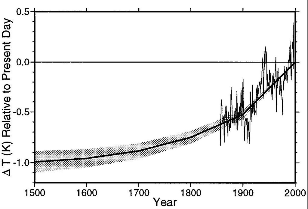 Now this reconstruction itself is under discussion, because it falls much lower than most other proxy records. They are also in disagreement with the various bent, broken or distorted hockey sticks which makes them quite popular some places. Mann, Rutherford, Bradley, Hughes and Keimeg took this on in 2003, (for those without access see comments in EOS I and EOS II
The low black line is Huang, et al. (2000) (a slightly updated version from the one shown above) averaging over the northern hemisphere. The dashed one areal weights the borehole data by cos-latitude. MRBHK2003 think that part of the story is that
The overwhelming majority of Northern Hemisphere borehole data come from regions that experience seasonal snow cover. The snow cover partially insulates the ground from cold-season air temperature and fluctuations therein, providing a potential insensitivity of the underlying ground temperature to cold winter air mass outbreaks (and implying a warm-season bias in borehole GST estimates, the degree of which depends on extent and duration of winter snow cover). Little, if any imprint, of the cooling associated with cold air outbreaks is recorded by a ground surface buried beneath a sufficiently thick seasonal snow cover layer. The accumulated influence of such outbreaks on winter mean SAT is considerably greater than the quite modest (on the order of a degree C or less) SAT trends sough from borehole reconstructions. In regions where midwinter snow cover has increased over the past few centuries (which could potentially be associated with either warmer or colder winters, depending on the details of air mass influence in the region), borehole GSTs may therefore exhibit a spurious apparent long-term warming (i.e., colder conditions back in time) due to an increasing incidence of insulating winter snow cover in more recent centuries.Without getting into the who is right who is wrong of this, we recently saw a reference to a new paper Pollack, H.N., Huang, S., Smerdon, J.E., 2006. Five centuries of climate change in Australia: The view from underground. Journal of Quaternary Science, 21 (7): 701-706. Now, if there is one place where it does not snow much, Australia is it. As big as Australia is, even including Tasmania, it goes from ~16 (cos = .96) to ~40 (cos = .77) degrees south, and the difference between the mean latitude and the max/min will only be ~ 10%, so at least two of the issues raised by MRBHK2003 (does that not just roll off the tongue), won't be very much there. Let us go to the video tape then and see how Pollack, Huang and Smerdon do on the MRBHK2003 scale

Follow the bright green line.......hmm. (I know, Australia is not in the northern hemisphere, but look look there is the little ice age. What more do you want from a poor bunny).


4 comments:
Thanks for getting back to me on Realclimate, Eli. I thought for a while I had committed some blogospheric faux pas and would never hear from anyone...
I hope I'm not being presumptuous, I'm just talking as someone plays with data a lot and knows how easy it is to make plausible models that fit the data we already have: the test is whether they have any predictive value. I posted the same question on the site of the fellow you call RPJ, where there was a discussion of various useful things one might like to predict (no reply there yet), so I am aware that the models should predict other things beside trends in global temperature.
So, were there predictions of high latitude warming being greater than low latitude, and stratospheric cooling, before these were experimentally observed, coming out of the models? Or could an antechinus like myself (I like your small furry animal persona, so will adopt one of my own) have predicted the observed effect by looking at the data available to the modellers and making a one-dimensional fit to the data?
F'rinstance, with your post of the 1st June, I think a rough and ready y=mx+c of T vs. ([CO2] a few decades earlier) fits 1998-2005 better than scenarios A, B , or C.
Basically, it bothers me that a ~1.* C rise has meant a 20 cm rise in sea-level, and people seem to blithely toss around 'metres' or 'tens of metres' as the result of a further 1-2 C. I presume this comes out of the models- but before I can join the bandwagon and call for drastic action to address global warming- action that might lead to people building a lot of nuclear power plants in my country, for example- I want to know, have the models made any successful predictions as non-intuitive as this before?
Pauli said that we have the equations to predict all of chemistry, the only problem is that they are too complicated to be soluble. This sounds bad, but it means that at least we know what a stable solution looks like. I'm worried that you guys aren't in as fortunate a position with your models.
I will read the stratospheric warming article properly, and heed your injunction to go forth and read more about climate models, I promise, just wanted to get back to you quickly!
Cheers,
Chris Fellows(latitude 30.8 S, elevation 1070 metres)
The first atmospheric models were one dimensional (altitude), however, in GCMs the C is for circulation, not climate. Climate and weather are inherently three dimensional, and the base of the models is solution of Navier-Stokes fluid dynamics equations. Stuff like real wind patterns pop out, for example. You can get some useful information from one dimensional models but it is quite limited (the stratospheric cooling is one of those things you can get from a 1D model). Even planetary (Titan, Venus, etc.) models today are two dimensional. Gas giants are easy, they have no surface. GCM resolution is not yet good enough to capture much surface detail, one of their weaknesses.
If you want an indication of how well these models do you can go get (J. Geo Res. 93 (1988) 9341)the Hansen GCM paper that people talk about, and compare their results with observed patterns of warming and other things. Some data is here http://www.giss.nasa.gov/research/news/20060925/ and there are data sets and model results here http://data.giss.nasa.gov/
Eli, as you said on RC about the Oz LIA - interesting.
Regards,
Paul Biggs
I'm not sure I totally follow your logic here, but comparing an AU reconstruction to the NH reconstruction from the MRBHK03 paper is entirely inappropriate. The timing and magnitude of climatic changes in the two hemispheres (let alone on the AU continent alone) can often be out of phase, of different magnitude, or both - depending on the time scales. This is clear from the comparison of the trends in the borehole recon and the surface air temperature in your modified figure - the trends in the green borehole recon match the NH SAT very poorly, while the NH borehole recon is well matched to the SAT trend. You should look closer at the AU study in which the boreholes compare well with the tree-ring reconstructions from NZ and Tasmania (standardized to preserve low-frequency variance). This regional agreement is promising and suggests that both the tree-ring and the boreholes preserve well the low-frequency variability of a region.
Regarding MRBHK03, you have unfortunately missed an important correction to the paper by the authors that was motivated by a critique by Pollack and Smerdon:
Pollack, H. N., and J. E. Smerdon (2004), Borehole climate reconstructions: Spatial structure and hemispheric averages, J. Geophys. Res., 109, D11106, doi:10.1029/2003JD004163.
Rutherford, S., and M. E. Mann (2004), Correction to ‘‘Optimal surface temperature reconstructions using terrestrial borehole data,’’ J. Geophys. Res., 109, D11107, doi:10.1029/2003JD004290.
In their correction, Rutherford and Mann admit to a mistake that overestimated the gridding effect by 40%. When this mistake is corrected, gridding is shown to make little difference (see the Pollack and Smerdon paper). The same mistake affected the optimal estimate in MRBHK03 derived from the EOF analysis...
Post a Comment