As Mr Dooley says, trust everyone, but cut the cards....

On second thought, maybe we should exclude Pat Michaels from that. More of a shake hands and count your fingers type that boy. A few weeks ago, I posted on a push back that had developed against Hansen, and his 1988 testimony to congress. A version of the key graph from Hansen's presentation, with the data up to 2000 is shown below (UPDATE: Eli substituted a new figure with observations updated until 2005 from PNAS: Global temperature change Hansen, Sato, et al. 2006 [5/11/07])

As you may recall, our boy Pat in later testimony to the US Congress, had erased the lines showing scenerios B and C and then claimed that Hansen's prediction was too high. In defense of Michaels, folk were claiming that Hansen had never said that scenerio B was the most likely. Eli went and RTFR (J. Geo Res. 93 (1988) 9341), and sure enough Hansen et al. sure enough said that B was the most likely scenerio

Now comes Paul Krugman, who as part of a column on the mendicity of the global warming denialists (Swift Boating the Planet), flat out calls Michaels a fraud, and takes Hansen to task for being unwilling to do so.

Even now, Dr. Hansen seems reluctant to say the obvious. "Is this treading close to scientific fraud?" he recently asked about Dr. Michaels's smear. The answer is no: it isn't "treading close," it's fraud pure and simple.

This, of couse, sets the cat among the canaries. Michaels posting from the Climate Change Denial Center of the world replied that he was sorely wounded, and then sets us off on a wild goose chase, commiting a second fraud.

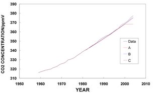
NASA scientist James Hansen had a model that did just this, published in 1988, and referred to in his June 23, 1988 Senate testimony as a “Business as Usual” (BAU) scenario.
BAU generally assumes no significant legislation and no major technological changes. It’s pretty safe to say that this was what happened in the succeeding ten years.
He had two other scenarios that were different, one that gradually reduced emissions, and one that stopped the growth of atmospheric carbon dioxide in 2000. But those weren’t germane to my discussion. Somehow, Krugman labelled my not referring to them as “fraud.”
The BAU scenario produced a whopping surface temperature rise of 0.45 degrees Celsius in the short period from 1988 through 1997, the last year for which there was annual data published by the United Nations’ Intergovernmental Panel on Climate Change at the time of my testimony. The observed rise was 0.11 degrees.
I cited the reasons for this. In fact, the rate of carbon dioxide increase in the atmosphere was quite constant–rather than itself increasing like compound interest–during the period.

The reason this is a fraud, is that there is very little difference up to 2004 in CO2 mixing ratios for Senerios A and B (and C tracks right along until 2000 when it goes flat). The graph below shows the data (Mauna Loa), and the predictions of Hansen's Scenerios A, B and C for CO2 concentrations.

(Click to enlarge and produce a clearer image)

Moreover, the assumptions of Hansen, et al. for the growth of CO2 concentrations was very good (both Scenerios A and B are about 2 ppm lower than measured in 2004). OTOH, we are now only about 18 years from the publication of the Hansen paper.

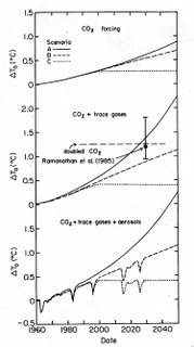
Until 2010, the difference in forcing between Hansens scenerios A and B all come from changes in concentration of chlorofluorocarbons, methane, and nitrous oxide and volcanic eruptions. You can see this in Fig. 2 from the paper. That figure shows (copy below) forcings from CO2 increases (top), CO2 + trace gases (middle) and CO2 + trace gases + aerosols from volcanos (bottom).

(Click to enlarge)

The dip in the bottom third near ~1982 represents the effect of the eruption of El Chichon, the later dips are guesses about when major eruptions will occur. Pinatubo came at in the 90s, a bit earlier than assumed, but the depth of the effect was about right.

So now the question is, how well did Scenerios A, B and C match the actual growth of concentrations of the other greenhouse gases and how well did the observed forcing match that assumed in each Scenerio. Unfortunately that means I have to find the observational data. Hints are allowed.

P.S. I see from Michaels post that RPJ has jumped the Hansen shark again.

On May 30, Roger Pielke, Jr., a highly esteemed researcher at University of Colorado’s Center for Science and Technology Policy Research, examined Hansen’s scenarios. Of the two “lower” ones, he concluded, “Neither is particularly accurate or realistic. Any conclusion that Hansen’s 1988 prediction got things right, necessarily must conclude that it got things right for the wrong reason.” (italics in original)

Well Roger, if you happen to peek in you can see that Hansen, Fung, Lacis, Rind, Lebedeff, Ruedy and Russell nailed the CO2 concentrations and the forcing from it.

Update: The emission scenerios for methane (CH4) are now posted.